Start with the relationship
The question this tool answers is specific: given coefficient, normal force, what value follows from the stated model? The result is expressed in N. The calculation below makes that relationship visible, so the answer can be checked independently instead of accepted as an unexplained number.
Choose a system boundary and a positive direction before entering measured values. Introductory equations deliberately leave out some real-world effects. If the setup has changing acceleration, drag, losses or nonuniform properties, first decide whether the simplified model is a useful approximation.
A worked example
Use the following values as a reproducible starting point. They are illustrative inputs, not measurements of your situation or a recommendation for a particular project. The calculator opens with the same values, making it possible to compare a manual calculation with the on-screen answer.
| Input | Example value | Unit |
|---|---|---|
| Coefficient | 0.3 | ratio |
| Normal force | 100 | N |
Substitute these quantities into the displayed relationship: coefficient = 0.3 ratio; normal force = 100 N. Carry out the operations before rounding the final value. This gives 30 N. The number is a result for this particular set of inputs; changing the measurement basis or the conditions can change its practical meaning.
What changes when an input changes?
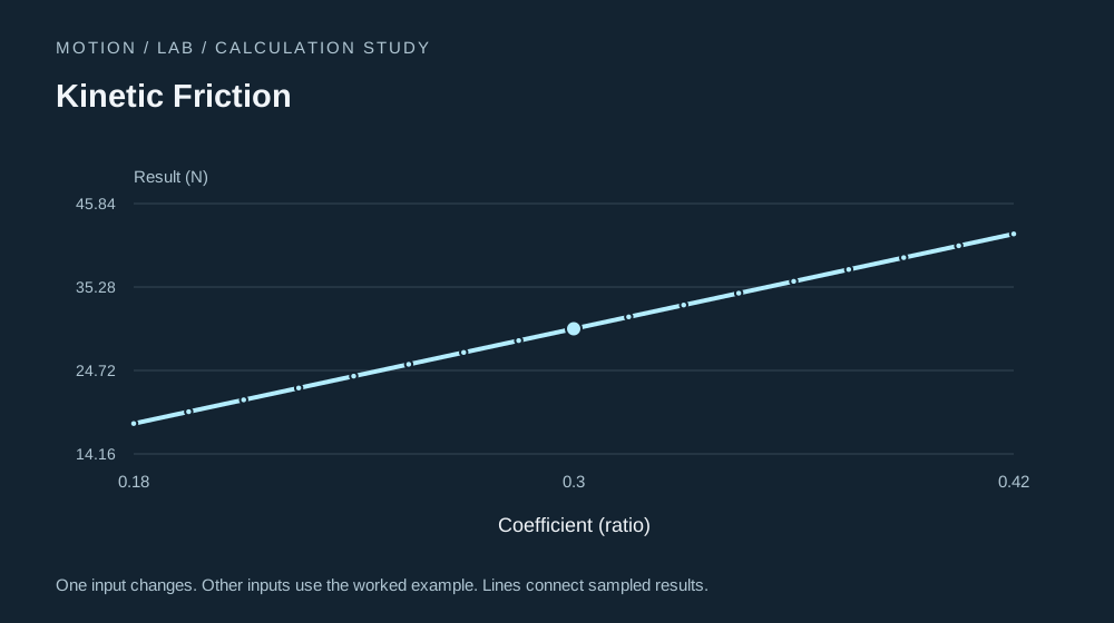
In the illustrated range, changing coefficient from 0.18 to 0.42 ratio moves the result from 18 to 42 N. The output increases between those endpoints. The table gives intermediate samples so you can see whether the response is smooth, stepped or nonmonotonic; the endpoints alone do not establish that behaviour.
Every other input keeps the value shown in the example table. This controlled comparison isolates one relationship at a time. For a real decision, try a lower, central and higher plausible input instead of treating an uncertain measurement as perfectly exact.
| Coefficient (ratio) | Result (N) |
|---|---|
| 0.18 | 18 |
| 0.24 | 24 |
| 0.3 | 30 |
| 0.36 | 36 |
| 0.42 | 42 |
The assumption that matters
The coefficient is empirical. Static friction and rolling resistance use different models.
A valid numerical result only means the entered values can be evaluated by this formula. It does not confirm that the formula describes every feature of the real situation. Read the unit labels, check the measurement method and keep the specific limitation above with the result when sharing it.
Use the result in your own work
Open the calculator, replace the example values and select Calculate. The result is evaluated on your device. Reset example restores this article's scenario, while Copy result keeps the quantity and unit together. If an input is outside the model's allowed range, correct it before interpreting the output.
Keep more digits during a chain of calculations than you show in a finished note. Displayed values are rounded for readability; extra decimals do not make a rough measurement more accurate. When your decision depends on a tight tolerance, compare the original measurements and assumptions before relying on the last displayed digit.
Further reading & method notes
OpenStax — mathematics and physics learning resources provides background for this subject. This article's numerical examples and chart were calculated from the formula shown above. See the editorial policy for how this collection presents assumptions and corrections.